Linearity: Why Batching Works

And the property that makes neural network training computationally tractable

📖 For the best reading experience with properly rendered equations, view this article on GitHub Pages.

---

Here’s something that should seem stranger than it does:

You can train a neural network on 1,000 samples almost as fast as on 10.

Not 100x slower. Almost the same speed.

How? The answer is a single property: linearity.

---

The Property

A function f is linear if:

f(αx + βy) = αf(x) + βf(y)

Scale the input, scale the output. Add inputs, add outputs. Combinations work as expected.

Matrix multiplication is the canonical linear operation:

f(x) = xW

Check: (αx + βy)W = αxW + βyW. ✓

This simple property is why modern deep learning is computationally tractable.

---

Why Batching Works

Consider a linear layer:

y = xW

For a single input x ∈ ℝ^(1×d_in) (a row vector), you get output y ∈ ℝ^(1×d_out).

Now consider a batch of n inputs, stacked as rows:

    ┌ x₁ ┐
X = │ x₂ │  ∈ ℝ^(n×d_in)
    │ ⋮  │
    └ xₙ ┘

The batched computation:

Y = XW

gives you all n outputs in one matrix multiply. Same W, same operation—just more rows.

This only works because the operation is linear.

If f weren’t linear, you couldn’t factor through the batch. You’d have to compute f(x₁), f(x₂), … separately.

But for linear operations, batching is free—mathematically. You’re computing the same thing, just organized differently.

---

Why GPUs Love Linearity

Matrix multiplication is the most optimized operation in computing.

• NVIDIA Tensor Cores: Designed specifically for GEMM (General Matrix Multiply)

• Memory bandwidth: Amortized across the batch

• Parallelism: Thousands of multiply-adds happening simultaneously

When you increase batch size:

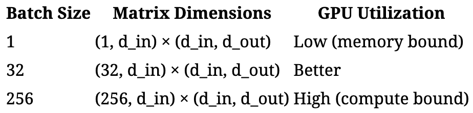
The weight matrix W is loaded once. Each additional sample in the batch is nearly free—you’re just doing more arithmetic while the data is already in fast memory.

Linearity turns “process n samples” into “one big matrix multiply.”

---

Gradient Accumulation

Here’s another consequence of linearity.

When you train on a batch, your loss is typically:

L = (1/n) Σᵢ Lᵢ

The gradient:

∇L = (1/n) Σᵢ ∇Lᵢ

Sum is linear. So:

• Compute gradients on samples 1-100, sum them

• Compute gradients on samples 101-200, sum them

• Add the partial sums

Same result as computing on all 200 at once.

This is gradient accumulation. When your batch doesn’t fit in memory, split it. Accumulate gradients across passes. Linearity guarantees correctness.

The same principle enables distributed training: compute gradients on different machines, sum them (all-reduce). Works because gradient aggregation is linear.

---

Why We Need Non-Linearity

If linearity is so great, why not make everything linear?

Because composition of linear functions is linear:

f(g(x)) = (xW_g)W_f = x(W_g W_f) = xW_combined

A 100-layer linear network equals a 1-layer linear network. No matter how deep you go, you can only learn linear functions.

Non-linearities create expressivity.

ReLU, GELU, softmax—these break linearity. They let deep networks approximate arbitrary functions.

The architecture of a neural network is:

Linear → Non-linear → Linear → Non-linear → ... → Linear

Linear operations: expensive, but batch-friendly, GPU-optimized. Non-linear operations: cheap (element-wise), parallel across the batch but no GEMM speedup.

This isn’t accidental. It’s engineered for hardware.

---

Where Linearity Breaks (And It Matters)

Batch Normalization

BatchNorm(x) = γ · (x - μ_B) / σ_B + β

The mean μ_B and standard deviation σ_B depend on which samples are in the batch.

Change the batch composition → change the normalization → change the output.

This is why:

• BatchNorm behaves differently in training vs. inference

• Small batches give noisy estimates

• BatchNorm can’t be cleanly gradient-accumulated

BatchNorm is not linear over the batch dimension.

Softmax in Attention

softmax(x)ᵢ = exp(xᵢ) / Σⱼ exp(xⱼ)

Every output depends on all inputs. You can’t compute softmax on parts and combine.

(Well, you can—that’s what we showed in the associativity article. But it requires the correction factor trick. It’s not trivially decomposable.)

Dropout

Stochastic. Different mask each time. Can’t be factored cleanly.

---

Backpropagation: Linearity of Differentiation

Here’s a deeper consequence.

Backpropagation relies on the chain rule:

∂L/∂x = ∂L/∂y · ∂y/∂x

But it also relies on differentiation being a linear operator:

∂/∂x(f + g) = ∂f/∂x + ∂g/∂x

∂/∂x(αf) = α · ∂f/∂x

Gradients add linearly. Scale linearly. This is why:

• Gradient of a sum = sum of gradients

• Gradient accumulation works

• Automatic differentiation is efficient

If differentiation weren’t linear, we couldn’t train neural networks.

The entire training paradigm—backprop, SGD, Adam—relies on gradients being linear in how they combine.

---

Practical Implications

Batch Size Tuning

Larger batches → better GPU utilization → faster per-sample processing.

But: larger batches can hurt generalization (sharper minima, less noise).

The trade-off is between:

• Hardware efficiency (wants large batches, because linearity makes them cheap)

• Optimization dynamics (sometimes wants smaller batches, for noise/regularization)

Gradient Checkpointing

To save memory, you can:

1. Discard intermediate activations during forward pass

2. Recompute them during backward pass

This works because the forward pass is deterministic—same input, same output. Recompute any segment, get identical activations, get identical gradients.

LoRA and Adapter Merging

Low-Rank Adaptation adds a small update:

W’ = W + BA

where B and A are low-rank matrices.

After training, you can merge the adapter back:

W_merged = W + BA

One matrix, no overhead at inference.

This works because matrix addition is linear. The adaptation is just a linear modification to the weights.

---

The Architecture of Efficiency

Modern neural networks are carefully designed around linearity:

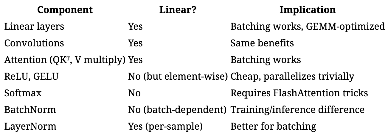
Notice the trend: we use LayerNorm instead of BatchNorm in Transformers. Why? LayerNorm normalizes within each sample, not across the batch. It’s linear over the batch dimension.

Architecture choices reflect the desire to preserve linearity where it matters.

---

The Takeaway

Linearity is why batching works.

f(batch) = batch of f

For linear operations, processing a batch is just one big matrix multiply. GPUs are optimized for exactly this.

This single property enables:

• Batched inference: 1000 samples nearly as fast as 1

• Batched training: gradients over many samples at once

• Gradient accumulation: split batches, sum gradients

• Distributed training: sum gradients across machines

• Backpropagation itself: gradients combine linearly

Neural networks are towers of linear operations with strategic non-linearities. The linear parts enable efficiency. The non-linear parts enable expressivity.

Lose linearity carelessly, and you lose the ability to batch. That’s why BatchNorm is tricky. That’s why softmax needed FlashAttention.

The algebra isn’t abstract. It’s why training is tractable at all.

Next in this series: Domain Transformations—why logarithms prevent underflow, why Fourier transforms speed up convolutions, and the art of finding easier spaces.

---

See also: The One Property That Makes FlashAttention Possible — Associativity is the license to parallelize, chunk, and stream.

---

Further Reading

• Why Momentum Really Works — Optimization dynamics and batch size

• A Survey of Quantization Methods — Linear error accumulation in approximate computation

• LoRA: Low-Rank Adaptation — Exploiting linearity for efficient fine-tuning

• Batch Normalization — And why it complicates things

Next in this series: Domain Transformations—why logarithms prevent underflow, why Fourier transforms speed up convolutions, and the art of finding easier spaces.